In classical computing, bits are the fundamental units of information, while quantum computing relies on qubits, mathematical entities that can be physically realized and exhibit unique properties. The development of a generalized theory of quantum computation and information can be achieved by considering qubits as abstract concepts, independent of any specific physical system.
Single qubit
A qubit, or quantum bit, can exist in states other than 0 or 1 and create linear combinations of those states. Mathematically, the state of a qubit can be represented as:
\[|\psi \rangle = \alpha |0 \rangle + \beta |1 \rangle\]Where $\alpha$ and $\beta$ are complex numbers such that $|\alpha|^2 + |\beta|^2 = 1$. When measured, only limited information about a qubit’s state can be obtained, with the probabilities of acquiring 0 or 1 adding up to one, i.e., $P(0) = |\alpha|^2$ and $P(1) = |\beta|^2$.
Quantum mechanics does not offer a straightforward relationship between its abstractions and reality, which makes understanding quantum systems’ behavior challenging. Nonetheless, the experimentally verifiable consequences of qubit states are crucial to the capabilities of quantum computation and information. Unlike classical bits, qubits can reside in any state between $|0\rangle$ and $|1\rangle$ until observed, and upon measurement, only ‘0’ or ‘1’ is returned as a probabilistic result.
Qubits are tangible entities that can be realized in various physical systems, such as photon polarization or electron states in atomic orbits. The Bloch sphere, a geometric representation, aids in visualizing a single qubit’s state in quantum computation and information. In this representation, the state of a qubit can be parameterized using two angles $\theta$ and $\phi$:
\[|\psi \rangle = \cos \frac{\theta}{2}|0 \rangle + e^{i\phi}\sin \frac{\theta}{2}|1 \rangle\]In theory, a qubit can store infinite information, but when measured, it collapses to either 0 or 1, yielding just one bit of information. Nature continuously maintains variables describing a qubit’s state, even when unmeasured, harboring concealed information. Grasping this hidden quantum information is vital for leveraging quantum mechanics in information processing.

Bloch Sphere
Python code
from qiskit.visualization import plot_bloch_vector
from qiskit.quantum_info import Statevector
from math import sin, cos
from cmath import exp
import matplotlib.pyplot as plt
from IPython.display import Image
import numpy as np

# Define the angles phi and theta
phi = np.pi / 2
theta = np.pi /4

# Convert the angles to Cartesian coordinates on the Bloch sphere
x = sin(theta) * cos(phi)
y = sin(theta) * sin(phi)
z = cos(theta)

# Create the statevector from the angles
state = Statevector.from_label('0') * cos(theta / 2) + Statevector.from_label('1') * exp(1j * phi) * sin(theta / 2)

# Plot the Bloch sphere
bloch_fig = plot_bloch_vector([x, y, z], coord_type='cartesian')

# Add custom labels for phi and theta
ax = bloch_fig.gca()
ax.text(x, y, z, f'$\\phi = {phi:.2f}, \\theta = {theta:.2f}$', fontsize=12)

# Save the plot to a file
bloch_fig.savefig("bloch_sphere.png", dpi=300)

# Display the saved image in the notebook
Image(filename="bloch_sphere.png")
Multiple qubits
A two-qubit system possesses four computational basis states and can exist in superpositions of these states:
\[|\psi \rangle = \sum_{i,j=0}^1 c_{ij}|i\rangle|j \rangle\]Where $c_{ij}$ are complex coefficients such that $\sum_{i,j=0}^{1}|c_{ij}|^2 = 1$. The measurement outcome probabilities are determined by each state’s associated complex coefficients, i.e., $P(i,j) = |c_{ij}|^2$.
The Bell state, also known as the EPR pair, is an essential two-qubit state in quantum computation and information, accounting for remarkable phenomena such as quantum teleportation and super-dense coding. The Bell state exhibits strong measurement correlations unattainable in classical systems, as evidenced by John Bell’s renowned result, highlighting the potential of quantum information processing to surpass classical limits.
The Bell state, an entangled two-qubit state, can be written as:
\[|\Psi^+ \rangle = \frac{1}{\sqrt{2}}(|00 \rangle + |11 \rangle)\]

Bell State
Python code
from qiskit import QuantumCircuit, QuantumRegister, ClassicalRegister
from qiskit.circuit.library import CXGate
from qiskit.visualization import circuit_drawer

# Create a quantum circuit with two qubits and two classical bits
qr = QuantumRegister(2)
cr = ClassicalRegister(2)
qc = QuantumCircuit(qr, cr)

# Add gates to create a Bell state
qc.h(qr[0])
qc.cx(qr[0], qr[1])

# Measure the qubits and store the results in the classical bits
qc.measure(qr, cr)

# Draw the circuit diagram
qc.draw(output='mpl')
Quantum systems comprising n qubits have $2^n$ amplitudes:
\[|\Psi \rangle = \sum_{i=0}^{2^n-1} c_{i}|i\rangle\]Where $c_i$ are complex coefficients such that $\sum_{i=0}^{2^n-1}|c_i|^2 = 1$.
Quantum systems comprising n qubits have $2^n$ amplitudes, where n=500 yields a larger number than the estimated number of atoms in the universe. Nevertheless, nature efficiently manages such vast data quantities, harnessing the immense computational power inherent in quantum mechanics.
Reference
Nielsen, M. A. & Chuang, I. L. Quantum Computation and Quantum Information. (Cambridge University Press, 2022).
Leave a comment